Normal Distribution Explained: Key Concepts And Uses

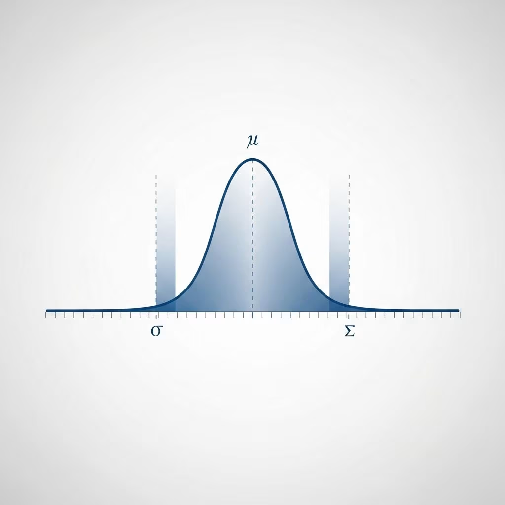
What Is Normal Distribution?

Normal distribution, also known as Gaussian distribution or the bell curve, is a continuous probability distribution that is symmetric about the mean. It represents one of the most important and widely used distributions in statistics and probability theory. In a normal distribution, data points tend to cluster around a central value, with the frequency of occurrences decreasing as you move away from the mean in either direction. This symmetry means that the distribution mirrors itself perfectly on both sides of the center point.

The normal distribution is fundamental to statistics because it describes how many natural phenomena distribute themselves in the real world. From heights of people to measurement errors and test scores, numerous variables follow a normal distribution pattern. The bell-shaped curve visually represents this distribution, showing how observations concentrate around the mean while becoming progressively rarer at the extremes.

Key Characteristics of Normal Distribution

Understanding the defining features of normal distribution is essential for applying it correctly in statistical analysis and data interpretation.

Symmetry Around the Mean

The normal distribution is perfectly symmetric around its mean (μ). This means that the left half of the distribution is a mirror image of the right half. Events or values that are equidistant from the mean have equal probabilities of occurring. This symmetry is one of the defining characteristics that makes the normal distribution so mathematically elegant and useful.

Mean, Median, and Mode Equality

In a normal distribution, three measures of central tendency—the mean, median, and mode—are all equal and located at the exact center of the distribution. The mean represents the average value, the median is the middle value when data is ordered, and the mode is the most frequently occurring value. Their equality at the center point reinforces the symmetric nature of the distribution.

Bell-Shaped Curve

The graphical representation of normal distribution is distinctly bell-shaped. The curve rises to a peak at the mean and then descends symmetrically in both directions. The highest point of the curve occurs at the mean, representing where the highest concentration of data points exists. This bell shape is why normal distribution is commonly referred to as the bell curve.

Mathematical Definition

The normal distribution is completely defined by two parameters: the mean (μ) and the standard deviation (σ). The mean determines the location or center of the distribution along the horizontal axis, while the standard deviation controls how spread out or concentrated the distribution is. Once these two values are specified, the entire distribution is fully determined.

Understanding the Empirical Rule (68-95-99.7 Rule)

The empirical rule, also known as the 68-95-99.7 rule or the three-sigma rule, is a critical concept for understanding how data distributes within a normal distribution. This rule provides a quick way to estimate the percentage of data that falls within a certain number of standard deviations from the mean.

The Three Levels of Standard Deviation

The empirical rule breaks down data distribution into three key intervals:

• One Standard Deviation (±1σ): Approximately 68% of all data falls within one standard deviation of the mean, meaning between μ – σ and μ + σ. This represents the central core of the distribution where the majority of observations concentrate.
• Two Standard Deviations (±2σ): Approximately 95% of all data falls within two standard deviations of the mean, between μ – 2σ and μ + 2σ. This wider interval captures nearly all meaningful observations in most datasets.
• Three Standard Deviations (±3σ): Approximately 99.7% of all data falls within three standard deviations of the mean. Values beyond this range are considered extreme outliers.

Practical Application of the Empirical Rule

Understanding these percentages helps analysts and researchers quickly assess data quality and identify outliers. If you have a dataset with a known mean and standard deviation, you can immediately determine what proportion of your data should fall into different ranges. This makes the empirical rule an invaluable tool for data analysis and quality control.

Mathematical Properties

Several important mathematical properties distinguish normal distribution from other probability distributions.

Probability Density Function

The normal distribution is defined by its probability density function, which describes the likelihood of observing specific values. The mathematical formula for the normal distribution probability density function is:

\[ f(x\mid \mu ,\sigma ^{2})={\frac {1}{\sigma \sqrt{2\pi}}}e^{-\frac{(x-\mu)^2}{2\sigma^2}} \]

This formula shows how the probability density depends on the distance from the mean, with the exponential function creating the characteristic bell shape.

Area Under the Curve

The total area under the normal distribution curve equals exactly 1, representing 100% of the probability. This fundamental property ensures that the probabilities of all possible outcomes sum to certainty. Any portion of the area under the curve represents the probability of values falling within that range.

Asymptotic Tails

The tails of a normal distribution curve are asymptotic, meaning they approach the horizontal axis but never actually touch it. Theoretically, the distribution extends infinitely in both directions, though the probability of values far from the mean becomes vanishingly small.

Real-World Applications of Normal Distribution

Normal distribution appears throughout nature and society, making it invaluable for analysis across numerous fields.

Common Examples

• Human Heights: The distribution of heights in a population typically follows a normal distribution, with most people clustering around the average height and fewer individuals at the extremes.
• Test Scores: Standardized test scores often approximate normal distributions, allowing educators and institutions to compare individual performance against population norms.
• Measurement Errors: Random errors in scientific measurements tend to distribute normally around the true value, which is why normal distribution is fundamental to error analysis.
• Blood Pressure: Blood pressure readings in populations typically follow a normal distribution pattern, helping medical professionals identify abnormal readings.
• Financial Returns: While not perfectly normal, many financial market returns approximate normal distributions over certain timeframes, enabling financial modeling and risk assessment.

The Central Limit Theorem Connection

Normal distribution forms the theoretical foundation of the Central Limit Theorem, one of statistics’ most powerful principles. The Central Limit Theorem states that the distribution of sample means approaches a normal distribution as the sample size increases, regardless of the underlying population distribution. This explains why normal distribution is so prevalent in statistical practice—when taking multiple samples and calculating their means, those means will tend toward a normal distribution even if the original data doesn’t perfectly follow one.

Standard Normal Distribution

The standard normal distribution is a special case where the mean equals 0 and the standard deviation equals 1. Any normal distribution can be converted to the standard normal distribution through a process called standardization, using the formula:

\[ Z = \frac{X – \mu}{\sigma} \]

This standardization allows researchers to compare values from different normal distributions on a common scale. Standard normal tables and calculators use this conversion to determine probabilities for any normal distribution.

When Normal Distribution May Not Apply

While normal distribution is widely applicable, it’s not suitable for all data types. Variables that are inherently positive or strongly skewed—such as income levels, asset prices, or reaction times—may not follow a normal distribution. In such cases, alternative distributions like the log-normal distribution or Pareto distribution may provide better models. Practitioners must evaluate whether normal distribution assumptions are reasonable before applying normal distribution-based statistical methods.

Advantages and Limitations

Advantages

• Mathematically well-understood and extensively studied
• Forms the basis for many statistical inference procedures
• The Central Limit Theorem ensures sample means approximate normality
• Simplifies complex analyses through standardization
• Applicable to numerous real-world phenomena

Limitations

• Not all data follows a normal distribution
• Presence of outliers can distort normal distribution assumptions
• Skewed or multi-modal data may violate normality
• May underestimate extreme events in financial data

Frequently Asked Questions

What is the difference between normal distribution and standard normal distribution?

Normal distribution is any distribution with a specific mean and standard deviation. Standard normal distribution is a special case with mean = 0 and standard deviation = 1. Any normal distribution can be converted to standard normal through standardization.

How do I know if my data follows a normal distribution?

You can assess normality using several methods: visual inspection through histograms and Q-Q plots, statistical tests like the Shapiro-Wilk or Kolmogorov-Smirnov tests, or calculating skewness and kurtosis values. Skewness near 0 and kurtosis near 3 suggest normality.

Why is normal distribution important in statistics?

Normal distribution is fundamental because many natural phenomena follow it, it forms the basis of the Central Limit Theorem, and it enables numerous statistical inference procedures. Most hypothesis tests and confidence intervals assume or rely on normal distribution properties.

Can I use normal distribution if my data is slightly skewed?

Depending on the degree of skewness and your analysis goals, slightly skewed data may still be acceptable. However, heavily skewed data violates normality assumptions and may require data transformation or alternative statistical methods.

What does the 68-95-99.7 rule tell me about my data?

This rule indicates how much data falls within specific standard deviation ranges. It allows you to quickly estimate what percentage of observations lie within one, two, or three standard deviations from the mean, helping identify outliers and assess data distribution.

This article is general information, not personal financial advice. Consider your own situation, or speak with a licensed adviser, before acting on it.

References

- Normal Distribution | Definition, Uses & Examples — GeeksforGeeks. 2024. https://www.geeksforgeeks.org/maths/normal-distribution/
- Normal distribution — Wikipedia. 2024. https://en.wikipedia.org/wiki/Normal_distribution
- Normal Distribution | Introduction to Statistics — JMP Statistical Software. 2024. https://www.jmp.com/en/statistics-knowledge-portal/measures-of-central-tendency-and-variability/normal-distribution